Note: This post was originally published on medium.
In the world of brick-and-mortar retail, gaining an edge on your competitors relies on both product and store management. Proper shift management requires a detailed understanding of store occupancy, the number of customers in your store through space and time. Historically, stores would gather occupancy data by paying an employee to stand outside and count the number of customers entering or exiting the store. Technology has advanced so that now stores can install custom cameras at store entrances and exits and automatically count customers. Unfortunately, the installation of these cameras is still cost-prohibitive. Even worse, errors from missed customers entering or exiting accumulate over time, making the counts inaccurate. The time is ripe for a next-gen approach to store occupancy models.
For my Insight Data Science project, I consulted with Brain of the Store (BotS). BotS wants to bring real-time artificial intelligence to brick-and-mortar retail by tracking customers in real time using computer vision (CV). Most retails stores already have surveillance cameras installed to survey the entire store. BotS analyzes real-time tracking data of the store employees and customers by partnering with a company that passes this pre-existing surveillance camera footage through CV algorithms. The partner company outputs coordinate data (x, y) linked to timestamps, which I call a track in this post. BotS then uses these tracks to build spatial and temporal models of store occupancy.
I aimed to fix some of the errors created from the computer vision process. The first and most obvious error of CV is track instability. A clear example of this would be someone who walked behind a pillar (relative to the camera view). When they walk behind the pillar, they are no longer identified by the CV and when they reappear they are given a new identification number. While this probably won’t have an effect on overall occupancy, the length of individual tracks becomes important in the second part of the project, specifically when two cameras identify the same person twice.
The multiple identification problem takes a little more explanation. Many stores use multiple cameras with overlapping coverage to get complete store coverage. If a person walked through both cameras’ fields of view at the same time, then our CV dataset would have duplicate tracks, thereby inflating the ultimate estimate of occupancy.
The original occupancy model
Before delving into my project, I want to set the stage and discuss what the raw models of occupancy look like. All of this data was collected from a cosmetics store in California.
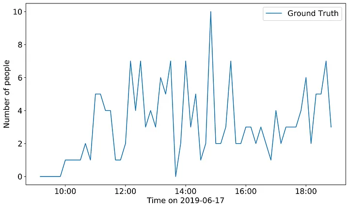
First, in order to understand how well CV estimates store occupancy, I needed a true value of store occupancy. BotS constructed this true value from the raw surveillance camera footage used for track construction and counted the number of people in the store at 10-minute intervals.
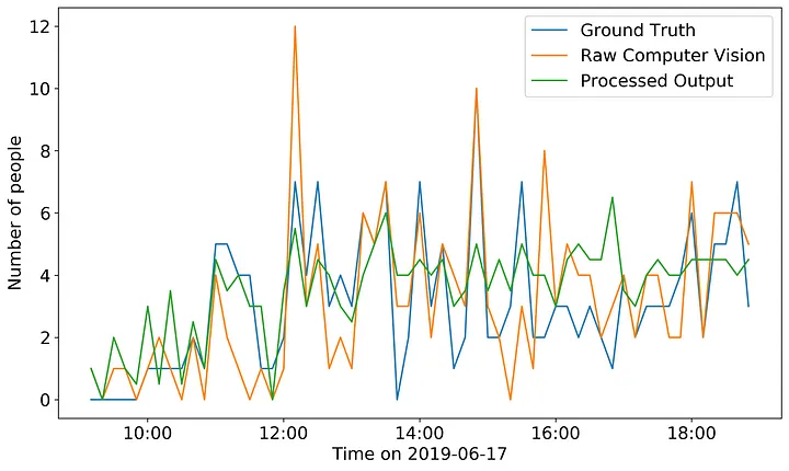
Then one of the BotS data scientists created an occupancy time-series model of the raw computer vision data alone.
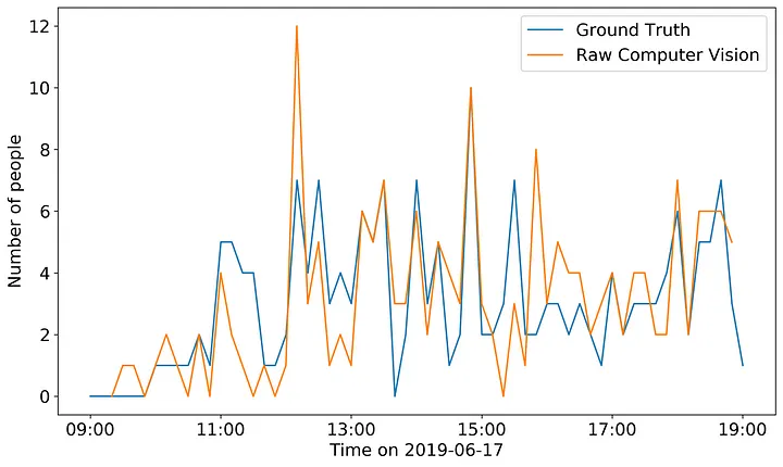
We can see from the figure above that the raw CV model underpredicts occupancy in some areas and overpredicts in others. The recall and precision of this model are 0.793 and 0.793 (respectively). I set out to use algorithmic methods to increase both the precision the recall of this model. I expected that my algorithms would reduce false positives by removing the duplicated tracks, and reduce false negatives by stitching tracks together during periods of time where no track existed previously (due to track instability).
A stitch in time
To figure out which tracks to stitch together, I made pairwise comparisons between each possible track. Before starting in on the explanation I need to define two terms: focal track and comparison track. The focal track is the first track in our pairwise comparison, the one that is ending. The comparison track is the track to which I am “comparing” the focal track. The comparison track is the second track, the one that is beginning. My overall plan was to compare the ending point of the focal track to the beginning of one (or more) comparison tracks. However, the ten hour dataset I used was large enough to cause some computational problems. I couldn’t just compare the ending and starting point of every track because with 30,776 tracks that would be over 900 million possible combinations!
Instead, I began subsetting the possible candidate tracks. First, I incorporated a time parameter that decided any track that started more than 1s after the focal track would be too delayed to be a possible stitching match. Then for each candidate track, I calculated the distance between the last point of the focal track and the first point of the candidate track. I then further subset the data by including a maximum distance parameter of 0.6 meters, because 76% of the candidate tracks were less than 0.6 meters from the focal track. Finally, I incorporated some characteristics of the focal track in making my comparison. I calculated the average speed of the focal track over the last 5 seconds and then estimated the possible distance the average speed could travel during the time separation between the focal and candidate track. While it is possible that someone could change their average velocity rapidly (imagine going from casually browsing the clearance section to running across the store) it is pretty unlikely.
After whittling down the potential candidate dataset using the process above, I conducted pairwise comparisons for each focal/candidate track pair. For each pair, I calculated the spacetime distance between the last point of the focal track and the first point of the candidate track. Spacetime distance sounds like a fancy concept, but really it is a three dimensional distance formula with the third dimension being time.
Equation 1: Spacetime distance formula given the differences in x-coordinates (x), y-coordinates (y) and time (t).
The advantage of using this formula is that it penalizes for both longer distances and longer time gaps. Any track that minimized the spacetime distance was then considered to be the final candidate track. Once I had the final candidate track, I linearly interpolated from the last point of the focal track to the first point of the final candidate track. Then I assigned all of the tracks the same ID as the focal track.
Seeing double
Once I stitched the tracks together I needed to address the problem of multiple identification. The cosmetic store client that BotS was working with had four cameras installed in its store. This means that each person could possibly be identified up to 4 times in the dataset!
To address this problem, I used another distance focused approach. Like the stitching problem, I first needed to reduce the potential comparisons.
The first step was to figure out which tracks were overlapping in time, since I was only interested in simultaneous co-identification. Then I further subset the data by only examining those tracks from different cameras. Consider two tracks that came from the same camera. Even if these two tracks are very close together, it is entirely possible that each of those tracks are a unique person, for example a mother and child would show up as two very close tracks in the same camera. Two tracks very close together but from different cameras are much less likely to be actually unique individuals.
For each overlapping track taken from a different camera, I calculated the Euclidean distance between each of the overlapping points in the focal and the comparison track. Then I calculated the average distance across both of the tracks. I considered comparison tracks that had an average distance of 0.8 m or less to be equivalent to the focal track. I estimated this distance as the approximate projection error between the different cameras.
More than one overlapping track could be flagged as the same, when this was the case, I set a decision rule to pick the longest track. While we may lose some information from the other tracks, the longest tracks will have the greatest information needed for the occupancy models.
Comparing occupancy models
What impact did these processing steps have? Recall that BotS is ultimately interested in constructing a time-series model of occupancy for this cosmetic store.
I calculated the expected occupancy of the store at each time step in my dataset by summing the number of tracks in a 5 minute window centered on the ground truth time point.
It is a little difficult to pull out the exact trends of my processed output versus the raw computer vision model. So I also plotted the difference of each from the ground-truth.
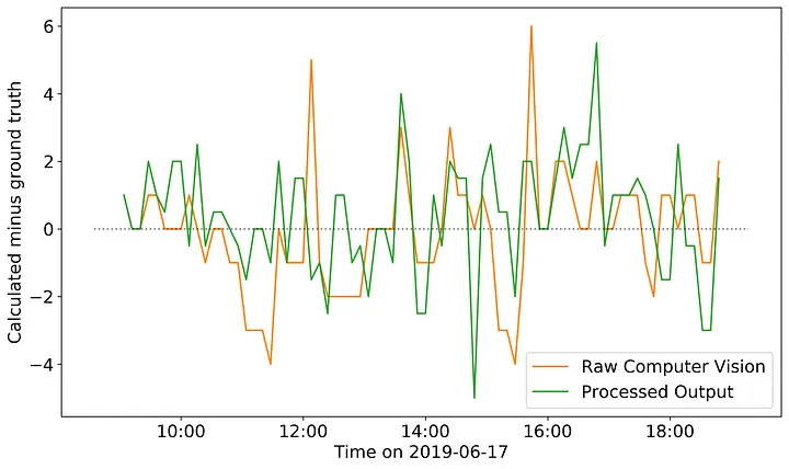
Here I can more clearly see the impact of my processed model compared to the raw CV occupancy model. The areas where the raw output tends to underpredict relative to the ground truth my processed model tends to overpredict. This result is reflected in the precision and recall of my model, 0.734 and 0.834 respectively. So while, I reduced the incidence of false negatives in my model, I increased the incidence of false positives. Therefore, I think what could work well for BotS is to create an ensemble prediction model using both the raw CV output and my processed model. By doing so, the areas where my model is more likely to overpredict would be balanced by where the raw model is more likely to underpredict, and vice versa.
Next Steps
There are a few parameters built into my algorithms where I could potentially build in some optimization. During the stitching step, the various parameters that subset the dataset could be optimized by finding locally stable regions where increases/decreases in the parameter would have no effect on the number of matches found. However, optimizing this parameter would be a time consuming process and so could only be done after an increase in computing power. A more likely optimization candidate would be during the multiple identification step. In this case, adjusting the maximum distance parameter, or changing the time threshold for comparison are both relatively inexpensive and could optimized for parameters with no local change in the number of candidate matches.
Beyond optimizing my algorithms, I think there are a lot of very interesting analyses that could be done with this dataset moving forward. For example, BotS could take the processed dataset and examine characteristics of each track for automatic identification of employees vs. customers. In theory, the track characteristic (velocity, headings between points) would be different for employees. A customer would be more likely to have a track that wanders throughout a store, while an employee would be more likely to make directed movements, or remain stationary for long periods of time (a cashier for example).
Regardless of the next steps, taking my processed model and developing a more accurate model of store occupancy will provide real value not only for BotS but for many brick-and-mortar retail stores.